Calculation of Gaussian Curvation via Connection Forms
In this article, I am going to calculate the Gaussian curvature via connection forms.
Suppose that 


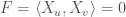


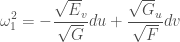
Let 


We obtain that
The Gauss-Codazzi equation tells us that
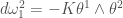
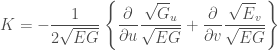
Hence
As an application, let us calculate the Gaussian curvature when the coordinate system is isothermal. Recall that a coordinate system 


